Activity 8: Enhancement in the Frequency Domain

The Fourier Transform is so powerful that it allows enhancing images in the frequency domain. The convolution theorem can be used to filter and mask unwanted frequencies in the frequency domain. The following activities show the prowess of the Fourier Transform:

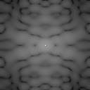
First I will showcase the two dots symmetrically along the x- axis and I take their Fourier Transform:

Figure 1

To generate the distance, I used the following code as a function of distance:

dist = 50
MAT = zeros(256,256);
MAT([128],[128 - dist, 128 +dist]) = 255,255;
Im = mat2gray(abs(fft2(MAT)));

As one can see, the frequency of the vertical lines increase as the distance between the 2 pixels increase. If I wanted horizontal lines, I would simply edit my code as follows:

dist = 50
MAT = zeros(256,256);
MAT([128 - dist, 128 + dist],[128,128]) = 255,255;
Im = mat2gray(abs(fft2(MAT)));

and get the following results:

Figure 2

I could make a checkerboard by changing MAT to:
MAT([128 - dist, 128 + dist],[128 + dist,128 + dist])

The next part of the activity shows an original (hand-drawn) image of two circles with a certain radius:

Figure 3

I take its FFT and get this:

Figure 4

The patterns look something from the Victorian era huh?

Now instead of circles, let's deal with squares, and see how the FFT vary in the frequency domain:

3 x 3 square (Left) and 5 x 5 square (right)

I manually input the squares locations at the center of the image. 

//Three by three Squares

N = 256

MAT2 = zeros(N,N);

MAT2([N/2 + 1,N/2 ,N/2 + 1],[N/2 - 11,N/2 - 10,N/2 - 9]) = [255,255,255;255,255,255;255,255,255];

MAT2([[N/2 + 1,N/2 ,N/2 + 1],[N/2 + 11,N/2 + 10,N/2 + 9]) = [255,255,255;255,255,255;255,255,255];

IM2 = mat2gray(abs(fft2(MAT2)));

imwrite(IM2, 'Squaredots.bmp');

imshow(IM2);

//Five by Five Squares

MAT3 = zeros(256,256);

MAT3([126,127,128,129,130],[116,117,118,119,120]) = 255*ones(5,5);

MAT3([126,127,128,129,130],[136,137,138,139,140]) = 255*ones(5,5);

IM3 = mat2gray(abs(fft2(MAT3)));

The code snippet above shows exactly how I manually input the squares. Note as one increases the size of the square, the greater the frequency of its FFT. On the next process, I will perform the FFT on ten randomly placed pixels on the image and convolve it with a square mask. The following shows the result:

Figure 6

As expected the results show the square mask displayed in the randomly generated area.

In the next part, 

//Convolution

A = zeros(200,200);

d = zeros(200,200);

Randomat = grand(10,2,"uin",0,200); //Generates the random locations of the numbers

for i = 1:1:10

     A(Randomat(i,1), Randomat(i,2) ) = 1;

end

five = rand(5,5);

d([98,99,100,101,102],[98,99,100,101,102])=five;

FTA = fft2(A);

Ftd = fft2(d);

FTAd = FTA.*Ftd;

IM4 = mat2gray(abs(fft2(FTAd)));

imwrite(IM4, 'RandConvol.bmp');

imshow(IM4);

Now we can do much more complicated filtering as in Figure 7. Here, we have a Lunar Orbiter Image with horizontal lines (left image):

Figure 7: Left image(Lunar Finding without Filter) Right image (Lunar Finding with Filter)

Figure 7: Left image(FFT of the image without the filter) Right image (FFT of the image with the filter)

The code snippet below shows how "elegantly," I generated the filter mask. Line 6 defines how much of the FFT image I remove with values ranging from 0 to 0.5. If I put 0.5, it removes everything, if I put 0, nothing happens. The best image is 0.49. The reason is that I apply the filter mask before the log, so the threshold is very small, as 0.48 and 0.49 are very distinct. The strength of this filter mask is that it can be applied on any image.

[1] //Lunar Landing Scanned Pictures: Line Removal

[2] Lunar = double(imread('C:\Users\Phil\Desktop\Academic Folder\Academic Folder 13-14 First Sem\AP 186\Activity 8\lun.jpg'));

[3] R = size(Lunar,1);

[4] C = size(Lunar,2);

[5] fftLunar = fftshift(fft2(Lunar));

[6] remov = 0.49;

[7] fftLunar(R/2 +1, 1:remov*C) = zeros(1,remov*C);

[8] fftLunar(R/2 +1,(1-remov)*C:C)= zeros(1,remov*C +1);

[9] fftLunar(1:remov*R,C/2 +1) = rand(remov*R,1);

[10] fftLunar((1-remov)*R:R,1+ C/2) = rand(remov*R+1,1);

[11] Im6 = mat2gray(abs(fft2(fftLunar)));

[12] imshow(Im6);

Note: Due to SPP and exams, I was unable to update the blog. The blog will continually be updated. Thank you!

Activity 7: Fourier Transform Model of Image Formation

Unlike the last activity in which I had such a hard time, this was more lenient, because Fourier Transforms are easy to deal with. Given a certain image, the Fourier Transform of the image in matrix form can be used to obtain its image in spatial frequency domain. The equation of the Fourier Transform can be divided into real and imaginary parts given by:

Figure 1

\

So  here Figure 1 shows an image of a circle with radius of 50% of total length of image or 64-bit radius. We take the Fourier transform and shift the image. Note we have to take the FFTshift or else the image will be just a dark figure. Figure 2 is the resulting image.

Figure 2

 Next we take the Fourier Transform of the letter "A." (Figure 3) The resulting Fourier Transform of Figure 3 is Figure 4. Take the Fourier Transform of Figure 4 again which is essentially taking the inverse Fourier Transform of figure 3 and we come back to the original image.

Figure 3

Figure 4

Figure 5

Next we perform convolution of two images. Convolution of two images is essentially the product of element per element of the two images in matrix form in inverse spatial frequency domain. Here the Fourier Transform is performed on the image VIP. It is then multiplied to a circle with an aperture of different radius. Since we are dealing with 128 bits, the circle is forced to have 128 x 128 elements. The elements are then multiplied to the Fourier transformed image. Figure 6 shows the resulting images.

Figure 6

The resulting image becomes unidentifiable as the aperture becomes smaller and smaller. Next we perform correlation. In correlation before multiplying two images element per element, the conjugate of one of the images in matrix form is taken in its frequency domain. Here Figure 7' s matrix is applied the function conj().

before element per element multiplication of the letter A. 

Figure 7

Figure 8

The result shows a sharp bright dot in which the letter A can be found. This is a great application in processing large image files and facial recognition. Its only downside is that the original image can no longer be used.

Edge Detection:

Another important application of Fourier Transform, is edge detection. By performing a convolution of 3 x 3 unit matrix and  an image, the edges of the image can be seen. At points where there is no change, the matrix gives a value of zero. When the matrix does change, the value is no longer zero. The following matrices are convolved against the same VIP image. The more variation there are in the matrix, the better the edge detection.

Figure 9

Here, I try to recreate the Sobel edge detection. Since most edge detection split their matrix operator into a horizontal and vertical component, I do exactly the same method.  The Gradient magnitude is then computed by [3]:

where Gx and Gy are the matrix operators shown in Figure 10. As you can see the resulting image gradient: the Sobel Gradient shows a very sharp line on the edge of the letters VIP!

Figure 10

I would give myself a 12 for this activity!!!

Code Snippet:

//Set-up

x = [-1: 0.0157480:1];

[X,Y] = meshgrid(x);

r = sqrt(X.^2 + Y.^2);

circle = zeros(size(X,1), size(X,2));

circle(find (r <=0.05)) = 1.0;

//imshow(circle);

A = double(rgb2gray(imread('C:\Users\Phil\Desktop\A.png')));

//imshow(A);

VIP = double(rgb2gray(imread('C:\Users\Phil\Desktop\VIP.png')));

//imshow(VIP);

Spain = double(rgb2gray(imread('C:\Users\Phil\Desktop\CorrelationC.png')));

//imshow(Spain)

//FFT Circle

r = fftshift(fft2(circle));

//imwrite(mat2gray(abs(r)), 'FFTCircle.bmp');

//FFT twice

s = fft2(fft2(circle));

//imwrite(mat2gray(abs(s)), 'FFTtwice.bmp');

//FFT Letter A

z = fftshift(fft2(A));

//imwrite(mat2gray(log(abs(z))),'FFTA.bmp');

t = fft2(fft2(A));

//imwrite(mat2gray(log(abs(t))),'InverseFFT.bmp');

//Convolution

FFTVIP = fft2(VIP); 

FFTCircle = fftshift(circle);

convolved = fft2(FFTVIP.*FFTCircle);

G = mat2gray(log(abs(convolved)));

//imwrite(G,'FFTConvolved0.05.bmp');

//Correlation

FFTA = fft2(A);

FFTSpain = fft2(Spain);

F = mat2gray(log(abs(fftshift(fft2(FFTA.*conj(FFTSpain))))));

//imwrite(F,"FFTCorrelation.bmp");

//Edge Detection

MAT = zeros(128,128);

MAT2 = zeros(128,128);

randomat = [-1,0,3;5,-2,-4;2,-1,-2];

submat = [-1,-1,-1;2,2,2;-1,-1,-1];

submat2 = [-2,1,-2;1,4,1;-2,1,-2];

submat3 = [0,1,0;1,-4,1;0,1,0];

submat4 = [3,-1,3;-1,-8,-1;3,-1,3];

submat5 = [-4,7,2;-8,-1,3;2,-2,1];

sobelx = [-1,0,1;-2,0,2;-1,0,1];

submat7 = [-0.25,0,0.25;0,0,0;0.25,0,-0.25];

sobely = [1,2,1;0,0,0;-1,-2,-1]

MAT([63 64 65], [63 64 65]) = sobely;

MAT2([63 64 65], [63 64 65]) = sobelx;

FFTVIP = fft2(VIP); 

FFTMAT = fft2(MAT);

FFTMAT2 = fft2(MAT2);

convolvedmatrx = fftshift(fft2(FFTVIP.*FFTMAT));

convolvedmatrx2 =fftshift(fft2(FFTVIP.*FFTMAT2));

H = mat2gray(abs(convolvedmatrx));

I = mat2gray(abs(convolvedmatrx2));

J = sqrt((H.*H) + (I.*I))

imwrite(J,'sobel.bmp');

imwrite(edge(VIP,'sobel'),'sobel2.bmp')

References:

1. Soriano, Jing Activity 7 Activity 7: Fourier Transform Model of Image Formation

2. http://www.csce.uark.edu/~jgauch/5683/notes/ch04a.pdf

http://en.wikipedia.org/wiki/Sobel_operator

Activity 6 Enhancement by Histogram Manipulation

First and foremost, I really, really had a hard time with this activity. I was messing up with the program left and right. Why? There were two parts that I had trouble with:

(Ignore my ranting here and skip to the introduction if you don't want to read this part)

1. The back-projecting of the pixels between the desired CDF and original CDF
2. Faster way of switching pixels in the image

Don't worry. This blog contains all the cheat codes so you won't spend the midnight oil like I did, so if you want some challenge DO NOT READ my blog... I'm just joking.

Introduction:

Images believe it or not have a distribution function. The pixels, specifically, make up the probability distribution function in which a histogram of the image can be created. Pixel colors range from 0 to 255. 0 being totally black and 255 being sharpest white. Between these two values, 254 shades of gray (no pun intended) can be technically observed.

Now let us talk about Histogram Manipulation!
Histogram manipulation is one way of improving the quality of an image, enhancing certain image features, or mimicking the responds of different systems such as the human eye.[1]

To this extent, one can take the probability density function (PDF) of an image by simply counting the number of times each pixel number ranging from 0-255 appeared in the image and plotting No. of pixels vs pixel (0-255). Then one can take the cumulative density function (CDF), which is essentially similar to the probability density function except for two things:

1. It's a cumulative, which means the pixel numbers are increasing.
2. The pixel number is normalized by dividing the y-axis value by the total number of pixel. This means the y-axis always ranges from 0 to 1.

This process can easily be done in scilab, since scilab allows easy conversion of images to a matrix of pixel numbers.
Another process which will be used is the back-projecting of a desired CDF to the orignal CDF of the image. It's similar to reshuffling the image pixels of your choosing by simply deciding what CDF to use.
This back-projection can be understood easily thanks to Mum Jing's figure shown below:

Figure 1 [1]

Now let's get started!

Since I recently watched Monsters University in theaters, I'm going to take the image of Michael "Mike" Wazowski, best friend of Sully. 

 Figure 2 [2]

 Figure 2

 

Figure 3: PDF (left) and CDF (right)

Note that the x-axis is Pixel from 0-255 and y-axis for the PDF is the occurrence of the specific pixel in the image and the y-axis for the CDF ranges from 0 to 1.

Now I'm going to make a CDF that is a straight line like this:

Figure 4

To do this we make use of the code that I tirelessly worked on:

(1)Image = imread('C:\Users\Phil\Desktop\MU.jpg');

(2)im = RGB2Gray(Image);

(3)imwrite(im,'MU.bmp');

(4)pixel = 255

(5) //CODE SNIPPET from: Mum Jing's blogspot of obtaining pixel color (0-255) from an image

(6)val=[];

(7)num=[];

(8)counter=1;

(9)for i=0:1:pixel 

(10)    [x,y]=find(im==i); //finds where im==i 

(11)   val(counter)=i; num(counter)=length(x); //find how many pixels of im have value of i 

(12)    counter=counter+1;

(13)end

(14)//End of Code Snippet

(15)[n,m] = size(im);

(16)nor = num/(n*m);

(17)mat1 = val';

(18)mat2 = nor';

(19)//plot(val, nor);

(20)mat3 = cumsum(mat2);//creates matrix containing both 0-255 and corresponding no.of pixels

(21)oldp = linspace(0,1,pixel+1); // creates a straight line y-axis value (desired CDF)

(22)//input1 = linspace(-10,10,pixel+1)

(23)//oldp = (1+exp(-1*input1))^-1

(24)newp = interp1(oldp, mat1, mat3,'nearest'); //

(25)newm = [mat1;mat3;mat1;oldp;newp];//0-255;0-1(currentCDF);0-255;0-1 (new CDF);0-255

(26)editim = im;

(27)// This part of the code backprojects/replaces the old pixels of the image to the new one.

(28)for i = 1:pixel  

(29)    editim(find(im==newm(1,i)))= newm(5,i); //

(30)end

(31)imwrite(editim,'EditedMU.bmp');

(32)[edity, editx] = imhist(editim);

(33)clf()

(34)plot(editx,edity/(n*m));

(35)sumedit = cumsum(edity/(n*m));

(36)clf();

(37)plot(editx,sumedit);

Tada!! Here is the resulting PDF:

Figure 5

And Figure 6 shows the resulting image. As you can see, there is a distinct difference between this image and the original. The contrast between white and black is greater. This can be attributed to the fact that linearity creates pixels counts which drop to zero (As seen from the PDF).

Therefore there is a loss of information...

Now let's try to create a sigmoid function, defined by:

Here is my poor attempt at trying to replicate the PDF curve of the sigmoid function using GIMP:

(Will still update. Discuss Code and Gimp.....)

References:

1. Soriano, Jing, Activity 6 Enhancement by Histogram Manipulation

2. http://blogcritics.org/movie-review-monsters-university-3/

Activity 5: Area Estimation for Images with Defined Edges

Finding an area of a 2-dimensional image has many practical applications. (cancer research, remote sensing, automated product inspection [1] ) The problem arises when the image is non-uniform and asymmetric. Think of a blob or a poorly drawn circle. One cannot measure the area so easily. The best way to measure the area of such images is with the use of Green's Theorem.

Green's Theorem relates a double integral to a line integral. Let Region R with contour taken in the counterclockwise direction with F1 and F2 be continuous everywhere and with continuous partial derivatives:

                      

Which can be reduced  by letting  pairs F1 = 0 and F2 = x and second pair  F1 = -y and F2 = 0 via averaging to:

The Green's Theorem now becomes summation of edge point products of xi, yi+1 and xi+1, yi.

In summary, the area of any closed figure regardless of shape can be computed via Green's Theorem.


To obtain the edges of the images Scilab has a library of functions which finds edges of single channel image:

edge(im,method)


The methods are: 

1. sobel- discrete differentiation operator, computing an approximation of the gradient of the image intensity function; the result of the Sobel operator is either the corresponding gradient vector or the norm of the vector. [2]
2. prewitt - similar to sobel operator
3. log - 
4. fftderiv - detects zero-crossing of the second-order directional derivative in the gradient direction [3]
5. canny - function described by the sum of four exponential terms, but can also be approximated by the first derivative of a Gaussian.[4]

The following methods will be examined. The edge-finding algorithm which computes closest to the theoretical image area will also be determined.

So here I created a 2-dimensional image of a circle: (from Activity 1 actually)

Figure 1

This image is 300 x 300 with a circle radius of 105 pixels.
The edge detection algorithms are applied on the image above and the following results are observed:

Figure 2

In terms of pixel count, the theoretical area of the circle is 3.4636e+4 pixels.
Now I will discuss the very interesting method on how I was able to compute the area of the circle via Green's Method. First I will show the algorithm/code snippet of the code:

(1)Edge1 = edge(Image, 'canny'); //sobel, prewitt,log,fftderiv,canny
(2)imshow(Edge1);
(3)imwrite(Edge1,'canny.bmp');
(4)[i,j] = find(Edge1); //locates coordinates of the edges
(5)xc = sum(i)/(size(i,2));  // locates center coodinates
(6)yc = sum(j)/(size(j,2));  // locates center coodinates
(7)x =j-xc;
(8)y =yc-i; //subtracts center coordinates to all edge coordinates 
(9)r = sqrt(x^2 + y^2) //computes radius
(10)theta = atan(y,x)*(180/3.14159);  //computes theta
(11)z = [theta; x; y; r]';// creates matrix containing theta, x and y edge coordinates, and radius and transposes them
(12)[C, I] = gsort(z(:,1),'r','i'); //sorts Theta 
(13)sorted = z(I,:) // creates Index and sorts Theta with x and y following it
(14)xiy = sum(sorted(1:size(sorted,1)-1,2).*sorted(2:size(sorted,1),3)) //Applies the Green Function
(15)xyi = sum(sorted(2:size(sorted,1),2).*sorted(1:size(sorted,1)-1,3))//Applies the Green Function
(16)Area = 0.5*(xiy - xyi)//Applies the Green Function Area Formula
(17)Area2 = 3.14158*(nx*0.35)^2 //Area of the Circle
(18)Error = 100*sqrt((Area-Area2)**2)/Area2

The code basically goes like this:
I locate the edge points (white pixels) and their coordinates. The coordinates are not x-y cartesian and uses row x column. Lines 7 and 8 compensate for this. I then compute the corresponding theta of the x and y coordinates. The list of angles are then matched with their respective x and y coordinates as in line 11, and the matrix is transposed for convenicence. Then here lines 12 and 13 are used. I found this code snippet online http://www.equalis.com/forums/posts.asp?group=&topic=302065&DGPCrPg=1&hhSearchTerms=&#Post302949, which allows me to sort rows by order of their column. Specifically I need the x and y coordinates sorted by increasing angle.
Finally, lines 14 and 15 computes the Green's function using equation 3. The sorted x and y coordinates are computed. I had a hard time implementing the Green's function. But in my opinion, this is the most elegant and simple method to do so. All thanks to the operator ".*" This operator multiplies the matrix element by element. Without the dot, an error occurs. 

After which the two areas are compared and here are the results:

Theoretical Area:  3.4636e+4
Area - % Error:

sobel-  33830.75 - 2.32%

prewitt - 34334.25 - 0.87%

log - 34386.25 -0.72%

fftderiv - 34334.25 -  0.87%

canny - 34328.28 - 0.89%

The results show that the "log" method seem to be the best method in determining the area of a given image. "sobel" method seem to be the worst. As one can see, the circle image formed in the "log" method is well-defined and most importantly continuous as compared to the "sobel" method which has some gaps in the circumference of the circle. For all intents and purposes, I will use "log" and "prewitt" method.

Here is my attempt to draw a PERFECT circle =P

Figure 3

Here is the edge finding method using "log:"

Figure 4

Here is the edge finding method using "prewitt:"

Figure 5

Area for the circle is 

43601.23 pixels -"log" method

43562.70 pixels - "prewitt" method

Conclusion:

I need to practice drawing my circles. XD

Now I want to measure the land area of our house in Cavite. So I take a google map image of our lot, which looks like this:

Figure 6

Erase the land area off the image via Paint:

Figure 7

Crop, then perform edge finding methods (prewitt and log) on the cropped image (142 x 104):

Figure 8

The new image is now this, which area can be easily computed:

Note that 76 pixels is equivalent to 10 meters (from the original image). Which means there is 0.1315789 meters per pixel  or  0.0173130 sq. meters per  square pixels.  The computed pixel area is 

10800.88 sq. pixels *0.0173130 = 186.99  sq. meters.

I cleaned off the area and recomputed:

10390.70 sq. pixels * 0.0173130 = 179.89419 sq. meters.
Our land area according to the blueprints from our Architect says its 180 sq. meter!!!!
Yay!!!
One of my favorite activities, I must say. I enjoyed coding this part...

References: 

1. Jing Soriano A5- Area estimation of images with defined edges 2013
2-5. wikipeida.org

Activity 4: Image Types and Formats

In this activity we will be dealing with different Image Types and Formats. Image Types come in four different types: 

a. Binary Images 

b. Grayscale Images: 

c. Truecolor Images

d. Indexed Images

Details:
Item Type: JPEG Image
Size: 1.10 MB
Dimensions: 1920 pixels x 1200 pixels
Horizontal Resolution: 96 dpi
Vertical resolution: 96 dpi
Bit Depth: 24

Anyway here is a camera image of my family's dog, Tami. The details are as follows.

Details:
Item Type: JPEG Image
Size: 3.00 MB
Dimensions: 4608 pixels x 3456 pixels
Horizontal Resolution: 180 dpi
Vertical resolution: 180 dpi
Bit Depth: 24
Resolution unit: 2
Color representation: sRGB
Compressed bits/pixel: 3

Camera maker: Canon

Camera model: Canon PowerShot A4000 IS

F-stop: f/3

Exposure time: 1/8 sec.

ISO speed: ISO-400

Exposure bias: 0 step

Focal length: 5 mm

Max. aperture: 3.15625

Metering mode: Pattern

Flash mode: No flash, compulsary

In this activity, we will be experimenting with different file formats. There are many file formats. File Formats are categorized as either Raster or Vector. Raster types describes the characteristics of each individual pixels. Vector formats, on the other hand contain a geometric description that can be rendered smoothly at any display size. [2]  Some popular Raster formats include: JPEG, TIFF, RAW, GIF, BMP, PNG, PAM, WEBP. Vector Format images need to be "rasterized" be displayed on digital monitors. Cathode Ray tube technology (such as in radars, video games, medical monitors) make heavy use of Vector formats. Examples of Vector formats include CGM (computer graphics metafile), SVG, and Gerber File formats.
The scope of this activity will unfortunately fall only on Raster file formats, specifically, PNG, JPEG, TIFF, and BMP.

Here is an image of Juggernaut Dota 2 hero originally in PNG file file, courtesy of http://kkcdn-static.kaskus.co.id/images/2012/07/30/1101061_20120730125032.png

Here is the same file converted to
a. JPEG
    Dimensions: 481 x 432
    Size: 39.3 KB
    Bit Depth: 24
b. GIF
    Dimensions: 481 x 432
    Size: 42.7 KB
    Bit Depth: 8
c. Bitmap Image - 24-bit
    Dimensions: 481 x 432
    Size: 205 KB
    Bit Depth: 8
d. Bitmap Image -  16 Color-bit
    Dimensions: 481 x 432
    Size: 103 KB
    Bit Depth: 4
e. Bitmap Image - Monochrome bitmap
    Dimensions: 481 x 432
    Size: 27 KB
    Bit Depth: 1

PNG or Portable Network Graphics supports lossless data compression. It was created to improve and replace GIF (Graphics Interchange Format). PNG is used for the 2D interlacing method, the cross-platform gamma correction, and the ability to make anti-aliased balls, buttons, text and other graphic elements. It is currently the most lossless data compression image file format on the web. PNG started in 1977 and 1978 when two Israeli researchers, Jacob Ziv and Abraham Lempel, first published a pair of papers on a new class of lossless data-compression algorithms, now collectively referred to as ``LZ77'' and ``LZ78.'[3]
In 1983, Terry Welch of Sperry (which later merged with Burroughs to form Unisys) developed a very fast variant of LZ78 called LZW.[3]
JPEG or Joint Photographic Experts Group images allow tradeoff between quality image and file size. JPEG allows 10:1 compression ratio. JPEG utilizes Discrete Cosine Transform which mathematically converts each frame from spatial (2D) domain to frequency domain.
GIF (Graphics Interchange Format) is a bitmap image format created in 1987. It was originally called 87a. Later, 89a added support for animation delays, transparent background color, and storage of application-specific metadata. [4] As of now all relevant patents have expired. GIF's are now widely used for its simple animation found in websites such as 9gag.

Sources:
1.http://web.archive.org/web/20080610170124/http://www.codersource.net/csharp_color_image_to_binary.aspx
2. A4 - Image Types and Formats 2013.pdf, Soriano, Jing
3. History of the Portable Network Graphics, Greg Roelofs, http://linuxgazette.net/issue13/png.html
4. Graphics Interchange Format, Version 89a, 1 July 1990 Retrieved 6 March 2009