Friday, August 16, 2013

Activity 11: Application of Binary Operations


From the past two activities, we were able to use morphological operators to reduce and enlarge images. Now we will use the same method to filter out noise of images and identify the characteristics of the elements of the image such as area, etc.

Figure 1 is a simulated Image of Normal Cells in the blood. As one can see, the area of the cells (in white) are relatively equal in size. One can easily segment them from the background image using a certain threshold. The problem would be the clumped circles.

Figure 1: Simulated Image of Normal Cells

Figure 1 was cropped into 6 different images each 256 x 256 pixels in width, length. The point is to locate the ROI which gives the best estimate of the area of the cells. Area??
Yes, essentially we are trying to compute the area of the cells. To do this we need to remove the clumped cells together and just obtain the average area of the individual cells.

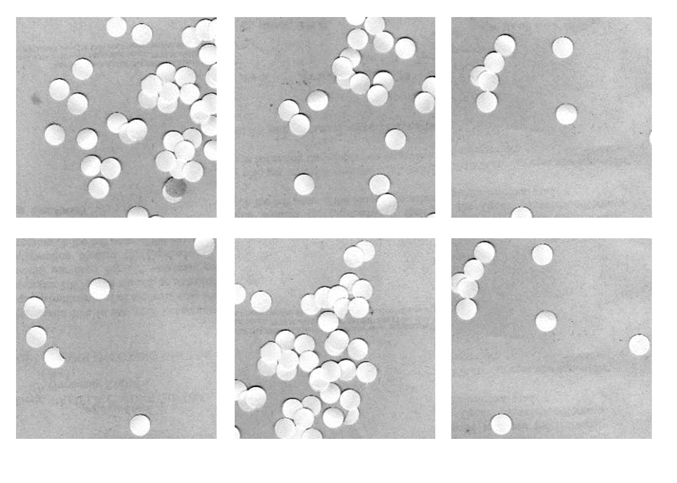
Figure 2: Six 256 x 256 pixels from Figure 1

The histogram was obtained to determine what threshold number will remove the unnecessary noise of the cell.

Figure 3: Histogram of each cropped image
 
Once the threshold was known, the cells were operated using the Opening and Closing Operator. It's apparent the threshold is around 200-240 form the histogram.

Closing Operator - retains light objects and removes dark objects the structuring element does not fit in. [2]
Opening Operator - retains dark objects and removes light objects the structuring element does not fit in [2]

The Opening operator was used to remove the small light objects and select only the larger ones. A structuring element of a circle was used.
 
Figure 4: Segmented with morphological operator
Figure 4 shows the resulting image. There are still  parts that need cleaning, but for the most they can be ignored. Image 6 (last image) needs cleaning up. 

I then computed the average area of the cells and took its standard deviation. Now there are times when SearchBlobs gives out a number 0 to a non-existing blobs, or the blob is so large that the standard dev is greater than the average! 

I figured a way or a workaround to this. I would re-run the loop, removing the abnormally large area (clumps of white cells), and recompute the area and standard deviation for each loop. I did this 3 times, in which I managed to decrease the standard deviation greatly. It's more of a cheat code I say.

Now, we use the computed areas of the normal cells, find them on the image with Cancer Cells. 
What I did was if the Blob (cell) was less than or equal to the computer area, then that blob is off the picture. I do this through the whole image until all the abnormally large cells or clumped up cells remain. 

Figure 5: Simulated Image with Cancer Cells
Figure 6 show the results. The best images are images 5 and 6. 

Figure 6: Image with only Cancer Cells 


bt = 0
for j = 1: 6
filename = 'C:\Users\Phil\Desktop\Academic Folder\Academic Folder 13-14 First Sem\AP 186\Activity 11\C1_0'+string(j)+'.jpg';
NormBC = double(imread(filename));
//Checks Histogram
pixel = max(NormBC);
val=[];
num=[];
counter=1;
for i=0:1:pixel 
    [x,y]=find(NormBC==i);
    val(counter)=i; num(counter)=length(x);
    counter=counter+1;
end
[n,m] = size(NormBC);
nor = num/(n*m);
plot(val,nor)
//Checks Histogram -endcode
Threshold = 200;
NormBC(find(NormBC<Threshold)) = 0;
StructureElement = CreateStructureElement('circle',5);
ResultImage = OpenImage(NormBC,StructureElement);
BinaryImage = SegmentByThreshold(ResultImage, CalculateOtsuThreshold(ResultImage));
//imshow(BinaryImage);
imwrite(BinaryImage,'C:\Users\Phil\Desktop\Academic Folder\Academic Folder 13-14 First Sem\AP 186\Activity 11\NormBC'+string(j)+'.jpg')
BlobImage = SearchBlobs(BinaryImage);
NumberofBlobs= max(BlobImage);
//imshow(mat2gray(BlobImage));
ct = 1
for i=1:1:NumberofBlobs
    Area(ct) = size(find(BlobImage == i),2);
    ct = ct+1;
end
average(j) = mean(Area);
sigma(j) = stdev(Area);
Area = Area(find(Area>0)); //eliminates annoying 0 blobs
at = 0
Checks = 3 //Does a re-computation of average and stdev after removing bad values
for l = 1:Checks
    X = Area(find(Area>(average(j)-sigma(j)) & Area<(average(j)+sigma(j))));
    clear average(j);
    clear sigma(j);
    clear Area(j);
    average(j) = mean(X);
    sigma(j) = stdev(X);
    Area = X;
    at = at +1;
end
Finalmean = mean(Area);
Finalsigma = stdev(Area)
ListofArea(j) = Finalmean;
Listofsigma(j)= Finalsigma;
end

//Cancer Blood Cells
CancerBC = double(imread('C:\Users\Phil\Desktop\Academic Folder\Academic Folder 13-14 First Sem\AP 186\Activity 11\Circles with cancer.jpg'));
CancerBC(find(CancerBC<Threshold)) = 0;
CancImage = OpenImage(CancerBC,StructureElement);
BinaryCancImage = SegmentByThreshold(CancImage, CalculateOtsuThreshold(CancImage));
imwrite(BinaryCancImage,'C:\Users\Phil\Desktop\Academic Folder\Academic Folder 13-14 First Sem\AP 186\Activity 11\CancBC.jpg');
Game = SearchBlobs(BinaryCancImage);
Cancerblobs = Game;
//imshow(mat2gray(Game));
NumberofCancBlobs= max(Cancerblobs);
dt = 1
for n=1: 6
    for m=1:1:NumberofCancBlobs
        if size(find(Cancerblobs == m),2) <= (ListofArea(n) + Listofsigma(n) )
            Cancerblobs(find(Cancerblobs == m)) = 0;
            h = m
        else
            Cancerblobs(find(Cancerblobs ==m)) = 255;
            z = m
        end
        dt = dt+1;
    end
    imwrite(mat2gray(Cancerblobs),'C:\Users\Phil\Desktop\Academic Folder\Academic Folder 13-14 First Sem\AP 186\Activity 11\FinalCancBC' +string(n)+'.jpg')
    clear Cancerblobs;
    Cancerblobs = Game;
end

References
[1] Soriano, Jing, Applications of Binary Operations 1: Blob Analysis, 2013
[2] SciLab 5.4.1 - Help Browser - Image Processing Design

Tuesday, August 13, 2013

Activity 10: Morphological Operations


So I've finally had the time to tackle this activity! I've finally posted the result of the Scilb images and code snippet. I will update the blog with my hand-drawn scans soon. Anyway on to the discussion:

Binary Images are just simply aggregates of 1's and 0's. This makes them easy to manipulate and extract information from them [1]. As such one can apply Set Theory. If you remember in Math 17, the first few topics are about sets, subsets, elements, etc, Well finally you can apply them here!

Now the table below is just a recall and basically a summary of Dr. Jing Soriano's review of Set Theory [1]:


With this, two morphological methods are used in processing binary matrices:
1.) Erosion - This essentially reduces the image to the shape of the STEL. (Structuring Element)

Mathematically, it can be represented as:

or visually:


2.) Dilation - This essentially expands/elongates the image to the shape of the STEL.

It can be mathematically represented as:
or visually:


Here is a video to further understand and visualize Dilation and Erosion [2,3] from: Smear lear's channel:


Dilation:


Erosion:


Scilab Code Snippet:
I generated the
//Square
Image1 = ones(8,8);
Image1(:,1)=0;
Image1(:,7)=0;
Image1(1,:)=0;
Image1(7,:)=0;
Image1(:,2)=0;
Image1(:,8)=0;
Image1(2,:)=0;
Image1(8,:)=0;
imwrite(Image1,'C:\Users\Phil\Desktop\Academic Folder\Academic Folder 13-14 First Sem\AP 186\Activity 10\5x5orig.bmp'); 

//Triangle
Image2 = zeros(7,7);
Image2(4,4)=1;
Image2(4,3)=1;
Image2(4,5)=1;
Image2(4,2)=1;
Image2(3,3)=1;
Image2(3,2)=1;
Image2(2,2)=1;
imwrite(Image2,'C:\Users\Phil\Desktop\Academic Folder\Academic Folder 13-14 First Sem\AP 186\Activity 10\triorig.bmp');


//Hollow Box
Image3 = zeros(12,12);
Image3(:,11) = 1;
Image3(:,2) = 1;
Image3(2,:) = 1;
Image3(11,:)= 1;
Image3(:,10) = 1;
Image3(:,3) = 1;
Image3(3,:) = 1;
Image3(10,:)= 1;
Image3(2,1)=0;
Image3(1,2)=0;
Image3(2,12)=0;
Image3(12,2)=0;
Image3(11,1)=0;
Image3(1,11)=0;
Image3(11,12)=0;
Image3(12,11)=0;
Image3(3,1)=0;
Image3(1,3)=0;
Image3(3,12)=0;
Image3(12,3)=0;
Image3(10,1)=0;
Image3(1,10)=0;
Image3(10,12)=0;
Image3(12,10)=0;
imwrite(Image3,'C:\Users\Phil\Desktop\Academic Folder\Academic Folder 13-14 First Sem\AP 186\Activity 10\hollorig.bmp');

//Cross 
Image4 = zeros(7,7);
Image4(:,4) =1;
Image4(4,:) = 1;
Image4(4,7)=0;
Image4(7,4)=0;
Image4(1,4)=0;
Image4(4,1)=0;
imwrite(Image4,'C:\Users\Phil\Desktop\Academic Folder\Academic Folder 13-14 First Sem\AP 186\Activity 10\crossorig.bmp');

MAT1 = [ %f %t %t;%f %t %t; %f %f %f];
MAT2 = [ %f %t %t;%f %f %f; %f %f %f];
MAT3 = [ %f %t %f;%f %t %f; %f %f %f];
MAT4 = [ %f %t %f;%t %t %t; %f %t %f];
MAT5 = [ %t %f %f;%f %t %f; %f %f %f];

imwrite(MAT1,'C:\Users\Phil\Desktop\Academic Folder\Academic Folder 13-14 First Sem\AP 186\Activity 10\2x2.bmp');
imwrite(MAT2,'C:\Users\Phil\Desktop\Academic Folder\Academic Folder 13-14 First Sem\AP 186\Activity 10\2x1.bmp');
imwrite(MAT3,'C:\Users\Phil\Desktop\Academic Folder\Academic Folder 13-14 First Sem\AP 186\Activity 10\1x2.bmp');
imwrite(MAT4,'C:\Users\Phil\Desktop\Academic Folder\Academic Folder 13-14 First Sem\AP 186\Activity 10\cross.bmp');
imwrite(MAT5,'C:\Users\Phil\Desktop\Academic Folder\Academic Folder 13-14 First Sem\AP 186\Activity 10\diag.bmp');

SE1 = CreateStructureElement('custom',[ %f %t %t;%f %t %t; %f %f %f]);
SE2 = CreateStructureElement('custom',[ %f %t %t;%f %f %f; %f %f %f]);
SE3 = CreateStructureElement('custom',[ %f %t %f;%f %t %f; %f %f %f]);
SE4 = CreateStructureElement('custom',[ %f %t %f;%t %t %t; %f %t %f]);
SE5 = CreateStructureElement('custom',[ %t %f %f;%f %t %f; %f %f %f]);
Rock = Image4
DI5x51 = DilateImage(Rock,SE1);
DI5x52 = DilateImage(Rock,SE2);
DI5x53 = DilateImage(Rock,SE3);
DI5x54 = DilateImage(Rock,SE4);
DI5x55 = DilateImage(Rock,SE5);
EI5x51 = ErodeImage(Rock,SE1);
EI5x52 = ErodeImage(Rock,SE2);
EI5x53 = ErodeImage(Rock,SE3);
EI5x54 = ErodeImage(Rock,SE4);
EI5x55 = ErodeImage(Rock,SE5);
imwrite(DI5x51,'C:\Users\Phil\Desktop\Academic Folder\Academic Folder 13-14 First Sem\AP 186\Activity 10\crossSE1.bmp');
imwrite(DI5x52,'C:\Users\Phil\Desktop\Academic Folder\Academic Folder 13-14 First Sem\AP 186\Activity 10\crossSE2.bmp');
imwrite(DI5x53,'C:\Users\Phil\Desktop\Academic Folder\Academic Folder 13-14 First Sem\AP 186\Activity 10\crossSE3.bmp');
imwrite(DI5x54,'C:\Users\Phil\Desktop\Academic Folder\Academic Folder 13-14 First Sem\AP 186\Activity 10\crossSE4.bmp');
imwrite(DI5x55,'C:\Users\Phil\Desktop\Academic Folder\Academic Folder 13-14 First Sem\AP 186\Activity 10\crossSE5.bmp');
imwrite(EI5x51,'C:\Users\Phil\Desktop\Academic Folder\Academic Folder 13-14 First Sem\AP 186\Activity 10\crossSE1Erode.bmp');
imwrite(EI5x52,'C:\Users\Phil\Desktop\Academic Folder\Academic Folder 13-14 First Sem\AP 186\Activity 10\crossSE2Erode.bmp');
imwrite(EI5x53,'C:\Users\Phil\Desktop\Academic Folder\Academic Folder 13-14 First Sem\AP 186\Activity 10\crossSE3Erode.bmp');
imwrite(EI5x54,'C:\Users\Phil\Desktop\Academic Folder\Academic Folder 13-14 First Sem\AP 186\Activity 10\crossSE4Erode.bmp');
imwrite(EI5x55,'C:\Users\Phil\Desktop\Academic Folder\Academic Folder 13-14 First Sem\AP 186\Activity 10\crossE5Erode.bmp');

UPDATE! Here are my hand-drawn scans. This was also good practice in preparation for the exams:


References:
[1]  Soriano, Ms. Jing, Activity 10 - Morphological Operations, 2013
[2] http://www.youtube.com/watch?v=fmyE7DiaIYQ
[3] http://www.youtube.com/watch?v=xO3ED27rMHs

Activity 9: Color Image Segmentation


I've finally been able to understand this Activity after hearing its discussion in the subject AP 187.Weird huh?

Anyway, when converting colored images (RGB) to grayscale, we lose valuable information. How do we minimize such losses? We can process the said image via "segmentation [1]."  The color of an object is actually a good description of its brightness and chromaticity. As such, instead of using RGB color space, we use NCC or normalized chromaticity coordinates.


There are two ways to do so, one is parametric and the other is non-parametric.
What are the steps in doing both? Simple, for parametric:
1. Crop a region of interest on the image.
2. Obtain the NCC of both the cropped image and whole image.
3. Compute the probability of the r and g values of the NCC in the cropped image and obtain its joint probability using:

4.  Compute the probability of the whole image.

For non-parametric:
1. Crop a region of interest on the image.
2. Obtain its 2-d histogram (which is essentially its PDF)
3.Back-project the binned histogram upon the whole image

Parametric has many assumptions. Its advantage is that it's useful for colors with different shadings. Non-parametric give finer control depending on the binning.


Parametric Image


Non-parametric

Code snippet:
ROI = double(imread('C:\Users\Phil\Desktop\Academic Folder\Academic Folder 13-14 First Sem\AP 186\Activity 9\ROI.png'));
Orig = double(imread('C:\Users\Phil\Desktop\Academic Folder\Academic Folder 13-14 First Sem\AP 186\Activity 9\Self.png'));
R = ROI(:,:,1);
G = ROI(:,:,2);
B = ROI(:,:,3);
I = R+G+B;
I(find(I==0))=100000;

Ri = Orig(:,:,1);
Gi = Orig(:,:,2);
Bi = Orig(:,:,3);
OI = Ri+Gi+Bi;
OI(find(OI==0))=100000;

ri = Ri./OI;
bi = Bi./OI;
gi = Gi./OI;

r = R./I;
g = G./I;

//Parametric 
meanr = mean(r);
meang = mean(g);
sigmar = stdev(r);
sigmag = stdev(g);

rp = (1/(sigmar*sqrt(2*%pi)))*exp(-((ri - meanr).^2)/(2*sigmar^2));
gp = (1/(sigmag*sqrt(2*%pi)))*exp(-((gi - meang).^2)/(2*sigmag^2));

rpgp = round(rp.*gp);
//imshow(rpgp);
imwrite(rpgp,'C:\Users\Phil\Desktop\Academic Folder\Academic Folder 13-14 First Sem\AP 186\Activity 9\Parametric.bmp')


//Non-Parametric

BINS = 32;
rint = round( r*(BINS-1) + 1);
gint = round (g*(BINS-1) + 1);
colors = gint(:) + (rint(:)-1)*BINS;
hist = zeros(BINS,BINS);
for row = 1:BINS
    for col = 1:(BINS-row+1)
    hist(row,col) = length( find(colors==( ((col + (row-1)*BINS)))));
    end;
end;
//imshow(hist);

//Backprojection
Nonpara = zeros(size(Orig,1),size(Orig,2));
for i=1:size(Orig,1)
    for j = 1:size(Orig,2)
        X = round(ri(i,j)*(BINS-1))+1;
        Y = round(gi(i,j)*(BINS-1))+1;
        Nonpara(i,j) = hist(X,Y);
    end   
end
imwrite(Nonpara,'C:\Users\Phil\Desktop\Academic Folder\Academic Folder 13-14 First Sem\AP 186\Activity 9\Non-parametric.bmp')

References:
[1]  Soriano, Jing, Activity 9 - Color Image Segmentation, 2013