Activity 15: Neural Networks

In the last activity, we used the average rgb of the image to either classify it as a basketball or football. We did not put into account of other images such as baseballs, or ping pong balls. Thus the method was rather crude.

In a Neural Network, one can ideally train the computer to respond to certain "stimulus" or characteristics/parameters of the image being process and label or flag it properly. The input or the "stimulus" activates the hidden response which is the weight. The weight is corrected by the test samples properly.

Figure 1: Diagram of a simplified Neural Network

In our activity we have 30 samples, 2 classes (basketball or football), and only 1 feature (subject to change). The shape and sizes of the balls are irrelevant since both are circular and their pixel area vary.



Code Snippet used[1]:

        // Simple NN that learns 'and' logic

// ensure the same starting point each time
rand('seed',0);

// network def.
//  - neurons per layer, including input
//2 neurons in the input layer, 2 in the hidden layer and 1 in the ouput layer
N  = [2,2,1];

// inputs
x = [1,0;
     0,1;
     0,0;
     1,1]';

// targets, 0 if there is at least one 0 and 1 if both inputs are 1
t = [0 0 0 1];
// learning rate is 2.5 and 0 is the threshold for the error tolerated by the network
lp = [2.5,0];

W = ann_FF_init(N);

// 400 training cyles
T = 400;
W = ann_FF_Std_online(x,t,N,W,lp,T); 
//x is the training t is the output W is the initialized weights, 
//N is the NN architecture, lp is the learning rate and T is the number of iterations

// full run
ann_FF_run(x,N,W) //the network N was tested using x as the test set, and W as the weights of the connections

//// encoder
//encoder = ann_FF_run(x,N,W,[2,2])
//// decoder
//decoder = ann_FF_run(encoder,N,W,[3,3])

References:
1. Soriano, Jing, Neural Networks, 2013

Activity 14 - Pattern Recognition

Humans are adept at recognizing patterns. We can identify the difference between cats and dogs, bananas and orange, cars and airplane. Children differentiate man and woman by their hairs. All of these have visual characteristics such as color and shape that allow us to differentiate one from another. Computers which can process information a lot faster than humans can be trained or programmed to recognize such patterns.

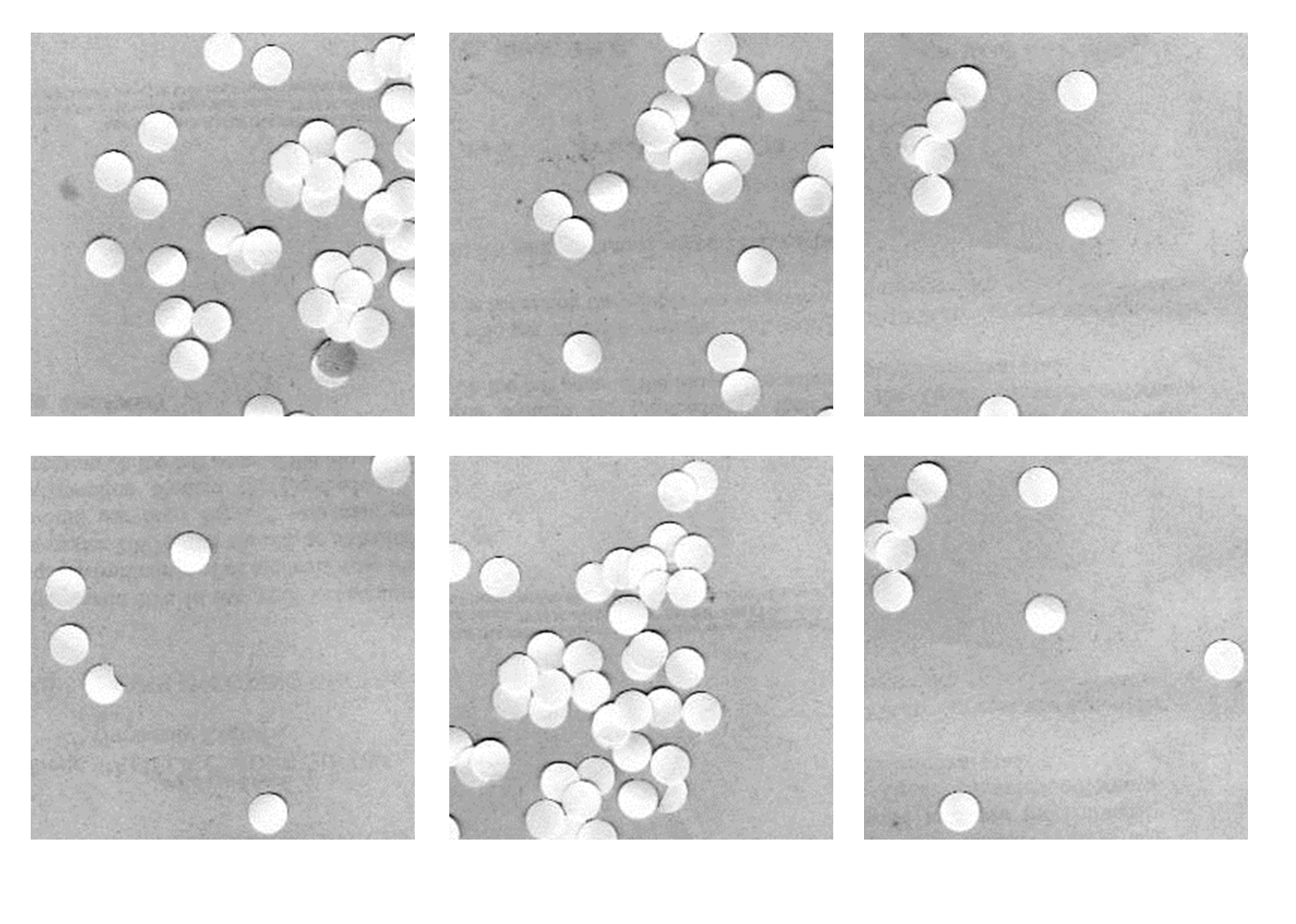
In this activity, 15 images of 200 x 200 pixels of soccer balls and basketballs are taken from google images. As such, it is the task of the program to differentiate the soccer balls from footballs. Figure 1 and 2 show the 30 images.

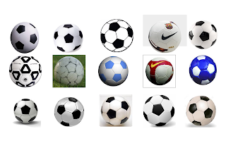
Figure 1: Fifteen Images of Soccer/Footballs

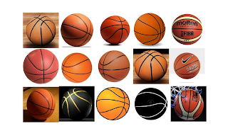
Figure 2: Fifteen Images of Basketball

The average rgb color of the images are taken per image. Their colors are then plotted. Figure 3 represents the image. The Green dots represent the average rgb of the basketball, and the blue dot represent the average rgb of the footballs.

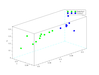
Figure 3: 3-D plot of trained images (both Basketball and Football)

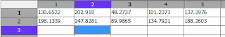
Figure 4: Distance plot between Test Basketball Images

From Figure 4, Row 1 represents the distance of the test basketball image against the trained basketball image. Row 2 represents the distance of the test basketball image against the trained soccer image. Evidently, for all columns, the distance of the trained basketball image is always smaller than the trained soccer image. This shows that the basketball images in terms of their rgb components is much closer to the color of the basketball which is exactly what we want. 

The result is 5/5 or 100% recognized. The weight of recognition however varies. 

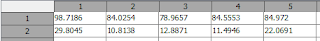
Figure 5: Distance plot between Test Soccer/Football Images

In Figure 5, same method was applied except the images are now trained football images. Row 1 represents the trained Basketball images and row 2 represents the trained soccer images. As shown, Row 2 is always less than Row 1. This means all images of the test scoccer are closer to the average trained soccer images.

The result is 5/5 or 100% of the images are recognized.

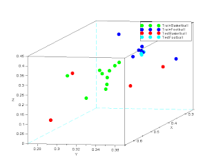
Figure 6: Location of the Test vs. Trained Images

Code Snippet:

//Training

Bred = [];

Bgreen = [];

Bblue = [];

for j = 1: 10

    filename = double(imread(['C:\Users\Phil\Desktop\Academic Folder\Academic Folder 13-14 First Sem\AP 186\Activity14\BasketBalls\Basket'+string(j)+'.jpg']));

    Bred = [Bred mean(filename(:,:,1))];

    Bgreen = [Bgreen mean(filename(:,:,2))];

    Bblue = [Bblue mean(filename(:,:,3))];

end

Bmeanrgb = Bred + Bblue + Bgreen;

param3d(Bred./Bmeanrgb,Bgreen./Bmeanrgb,Bblue./Bmeanrgb);

B = get('hdl');

B.foreground = 6;

B.line_mode = 'off';

B.mark_mode = 'on';

B.mark_size = 1;

B.mark_foreground = 3;

Sred = [];

Sgreen = [];

Sblue =[];

for j = 1: 10

    filename = double(imread(['C:\Users\Phil\Desktop\Academic Folder\Academic Folder 13-14 First Sem\AP 186\Activity14\SoccerBalls\Football'+string(j)+'.jpg']));

    Sred = [Sred mean(filename(:,:,1))];

    Sgreen = [Sgreen mean(filename(:,:,2))];

    Sblue = [Sblue mean(filename(:,:,3))];

end

Smeanrgb = Sred + Sblue + Sgreen;

param3d(Sred./Smeanrgb,Sgreen./Smeanrgb,Sblue./Smeanrgb);

B = get('hdl');

B.foreground = 6;

B.line_mode = 'off';

B.mark_mode = 'on';

B.mark_size = 1;

B.mark_foreground = 2;

hl=legend(['Basketball';'Football';])

Bmean = mean(Bred)+mean(Bgreen)+mean(Bblue);

Smean = mean(Sred)+mean(Sgreen)+mean(Sblue);

//Testing

BB = [];

SB = [];

Bredt = [];

Bgreent = [];

Bbluet = [];

for j = 11: 15

    filename = double(imread(['C:\Users\Phil\Desktop\Academic Folder\Academic Folder 13-14 First Sem\AP 186\Activity14\BasketBalls\Basket'+string(j)+'.jpg']));

    BB = [BB sqrt((mean(filename(:,:,1))-mean(Bred))^2 + (mean(filename(:,:,2)-mean(Bgreen)))^2+(mean(filename(:,:,3)-mean(Bblue)))^2)];

    SB = [SB sqrt((mean(filename(:,:,1))-mean(Sred))^2 + (mean(filename(:,:,2)-mean(Sgreen)))^2+(mean(filename(:,:,3)-mean(Sblue)))^2)];

    Comparison1= [BB;SB];

    Bredt = [Bredt mean(filename(:,:,1))];

    Bgreent = [Bgreent mean(filename(:,:,2))];

    Bbluet = [Bbluet mean(filename(:,:,3))]; 

end

Bmeanrgbt = Bredt + Bbluet + Bgreent;

param3d(Bredt./Bmeanrgbt,Bgreent./Bmeanrgbt,Bbluet./Bmeanrgbt);

B = get('hdl');

B.foreground = 6;

B.line_mode = 'off';

B.mark_mode = 'on';

B.mark_size = 1;

B.mark_foreground = 5;

Sredt = [];

Sgreent = [];

Sbluet = [];

BS = [];

SS = [];

for j = 11: 15

    filename = double(imread(['C:\Users\Phil\Desktop\Academic Folder\Academic Folder 13-14 First Sem\AP 186\Activity14\SoccerBalls\Football'+string(j)+'.jpg']));

    BS = [BS sqrt((mean(filename(:,:,1))-mean(Bred))^2 + (mean(filename(:,:,2)-mean(Bgreen)))^2+(mean(filename(:,:,3)-mean(Bblue)))^2)];

    SS = [SS sqrt((mean(filename(:,:,1))-mean(Sred))^2 + (mean(filename(:,:,2)-mean(Sgreen)))^2+(mean(filename(:,:,3)-mean(Sblue)))^2)];

    Comparison2 = [BS;SS]; 

    Sredt = [Sredt mean(filename(:,:,1))];

    Sgreent = [Sgreent mean(filename(:,:,2))];

    Sbluet = [Sbluet mean(filename(:,:,3))];

end

Smeanrgbt = Sredt + Sbluet + Sgreent;

param3d(Sredt./Smeanrgbt,Sgreent./Smeanrgbt,Sbluet./Smeanrgbt);

B = get('hdl');

B.foreground = 6;

B.line_mode = 'off';

B.mark_mode = 'on';

B.mark_size = 1;

B.mark_foreground = 4;

h2=legend(['TrainBasketball';'TrainFootball';'TestBasketball';'TestFootball'])

References:

1. Soriano, Jing, Act14 Pattern Recognition, 2013

Activity 13 - Image Compression

Now we tackle how jpeg/JPG images are compressed, and why it's one of the more popular image file formats used everywhere!

So first we need to understand how images are compressed.
JPEG images are usually split into blocks of 8 pixels. [1] They undergo the Discrete Cosine Transform (DCT), which is essentially the Fourier Transform but without the sine counter part. (only real values)
The following equation show the Cosine Transform:

We will try to simulate the Fourier Transform, by obtaining the Principal Components (PC) of an image.
This is done using the code below:

[lambda,facpr,comprinc] = pca(x);

The main use of this is to split the image into its eigenvalues and eigenvectors. From there we can reconstruct the image using only certain components of the image, without having to use the entire picture.

So our 1st step is to split the image into 10 x 10 pixels. This is easily done with the code given by Mum Jing:

I = imread('C:\Users\Phil\Desktop\Academic Folder\Academic Folder 13-14 First Sem\AP 186\Activity13\SF3.jpg');
I = im2double((I(:,:,1)+I(:,:,2)+I(:,:,3))/3);
//scf(); imshow(I);
//chop image into 10x10 blocks and assemble in a matrix x
clear x;
k=0;
for r = 1:8 //rows divided by block length
for c = 1:6 //columns divided by block width
itemp = I(((10*r-9):(10*r)),((10*c-9):(10*c)));
xtemp = itemp(:);
k = c + (r-1)*6;
x(k,:) = xtemp';
end

end

The image I will be using is a cropped image of the Dota 2 Hero Shadow Fiend:

Courtesy of biggreenpepper from deviantart website: http://biggreenpepper.deviantart.com/art/dota2-Shadow-Fiend-363299573

I crop the image into 80 x 60 pixels. I then use subdivide it into smaller matrices of 10x10.

I then take the PCA of these images and obtain the components of the image.

After which I reconstruct the image in grayscale.

Here is the image in its component form (a simulation of the Cosine Transform):

The following images are reconstructed of Shadow Fiends mouth.

Finally Shadow Fiend reconstructed at 90% corresponding to 50 coefficients and 100% at 100 coefficients!

Code Snippet used all thanks to Mum Jing!

//program to use pca for images

stacksize(10000000);

//load image and convert to grayscale

I = imread('C:\Users\Phil\Desktop\Academic Folder\Academic Folder 13-14 First Sem\AP 186\Activity13\SF.jpg');

I = im2double((I(:,:,1)+I(:,:,2)+I(:,:,3))/3);

I2 = mat2gray(I);

imwrite(I2,'C:\Users\Phil\Desktop\Academic Folder\Academic Folder 13-14 First Sem\AP 186\Activity13\ORIGSF.jpg');

//chop image into 10x10 blocks and assemble in a matrix x

clear x;

k=0;

[S,T] = size(I);

for r = 1:(S/10) //rows divided by block length

for c = 1: (T/10)//columns divided by block width

itemp = I(((10*r-9):(10*r)),((10*c-9):(10*c)));

xtemp = itemp(:);

k = c + (r-1)*(T/10);

x(k,:) = xtemp';

end

end

// apply pc to set x

//clear lambda, facpr, comprinc

[lambda,facpr,comprinc] = pca(x);

//test reconstruction- display pc's

VARY = 30;

coef = comprinc(:,1:VARY)';

EI = facpr(:,1:VARY);

IM1 = EI*coef;

//imshow(IM1);

y = zeros(S,T);

k=0;

for r = 1:(S/10)

    for c = 1:(T/10)

        k = c + (r-1)*(T/10);

        xtemp=IM1(:,k);

        y(((10*r-9):(10*r)),((10*c-9):(10*c))) = matrix(xtemp,10,10);

    end

end

imshow(y);

imwrite(y,'C:\Users\Phil\Desktop\Academic Folder\Academic Folder 13-14 First Sem\AP 186\Activity13\NEWSF3.jpg');

//newcomprinc = zeros(100,T)

// Normalizes EigenVector

//for j = 1:T

//    newcomprinc(:,j) = comprinc(:,j)/sqrt(sum(comprinc(:,j)^2))

//end

//scf();

//imshow(Recon);

//

I would give myself a 12 for this activity for I was able to also generalize the code for all sizes of the image!!

References

[1] Soriano, Jing ACT 13 - Image Compression, 2013

Activity 12: Playing Notes by Image Processing

Another great application of image processing is the ability to convert image into sounds. Say, I have a musical sheet in an image format. I can use morphological filters to isolate the musical notes, use the location of these notes, convert the location of these notes to frequency, and essentially play these notes!

Here, I have a song sheet for Twinkle Twinkle Little Star, one of the easiest songs to play on the piano.

Here is the note musical note placed in one single line to make image processing easier. This at least normalizes the y- coordinate plane.

Then I use the code snippet below:
[Row,Column] = size(MS);
SE1 = CreateStructureElement('vertical_line',3);
SE2 = CreateStructureElement('horizontal_line',2);
A = ErodeImage(~MS, SE1); //Removes Horizontal lines
B = ErodeImage(A, SE2);  //Removes Vertical Lines
imwrite(mat2gray(B),'C:\Users\Phil\Desktop\Academic Folder\Academic Folder 13-14 First Sem\AP 186\Activity 12\MorpedTwinkle.png');
BlobImage = SearchBlobs(B);
NumberofBlogs = max(SearchBlobs(B));
IsCalculated = CreateFeatureStruct(%f);
IsCalculated.Centroid = %t

BlobStatistics = AnalyzeBlobs(BlobImage,IsCalculated);
ct = 1
for i=1:NumberofBlogs
    xc(ct) = BlobStatistics(i).Centroid(1);
    yc(ct) = BlobStatistics(i).Centroid(2);
    Area(ct) = size(find(BlobImage==i),2);
    ct = ct + 1;
end

to remove the horizontal and vertical lines on the song sheet. I thus get the location of each notes, using the remaining blobs.

I then plot the remaining plot in its x and y coordinates, and do the following conversion there:

As one can see, both graphs are similar which is exactly what I need. The frequencies are then played using the code snippet used:

function n = note(f, t)

n = sin (2*%pi*f*t);

endfunction;

//Notes 1st Octave

R = 0;

G0 = 196.00*2;

A0 = 220.00*2;

B0 = 246.94*2; 

C0 = 261.63*2;

D0 = 293.66*2;

E0 = 329.63*2;

F0 = 349.23*2;

G0 = 392.00*2;

//Notes 2nd Octave

G1 = 196.00*4;

A1 = 220.00*4;

B1 = 246.94*4; 

C1 = 261.63*4;

D1 = 293.66*4;

E1 = 329.63*4;

F1 = 349.23*4;

G1 = 392.00*4;

//Durations 

EN = soundsec(0.125) //Eigth note

QN = soundsec(0.25); //quarter note

HN = soundsec(0.5); //Half note

FR = soundsec(1.); //Full note

I was able to convert the y - length successfully using the code snippet below:

But the x-length conversion needs clean-up. Up to now I was able to successfully convert the x-length to matrix, but when I convert the numbers into soundsec(), the matrices have different sizes which I have yet to bypass.

//Converts Y length to note value

yn = yc;

sens = 0.02; //Sets sensitvity  

yn(find(yn<0.15 +sens & yn> 0.15-sens)) = C0;

yn(find(yn<0.382 +sens & yn> 0.382-sens)) = G0;

yn(find(yn<0.436 +sens & yn> 0.436-sens)) = A1;

yn(find(yn<0.317 +sens & yn> 0.317-sens)) = F0;

yn(find(yn<0.271 +sens & yn> 0.271-sens)) = E0;

yn(find(yn<0.214 +sens & yn> 0.214-sens)) = D0;

//Converts X length to note value

for k=1:length(xc)-1

    xc(k) = xc(k) - xc(k+1)

end

xn = xc

xn(find(xn>=0.033)) = 0.5;

xn(find(xn<0.033)) = 0.25;

game = [];

for j=1:length(yn)

    game($+1,:) = note(yn(j),soundsec(0.5));

    end

SOUND = matrix(game', 1, length(game));

sound(SOUND);

Anyhow, here is the resulting sound in .mp4 format:

References:
1. Jing, Soriano - Playing notes by Image Processing, 2013

I would give myself a 10 for this activity due to the fact that I was able to use Morphological Filters to play notes in Scilab. I would love to update the code to be able to

1. Play any musical sheet, which means that I don't have to edit the song sheet
2. Increase the dictionary of the code. That means include eighth notes, rests, sharps, etc.
3. Ability to use the area of the blob to also determine the length. This particularly useful for half notes, which I t put to use...

Activity 11: Application of Binary Operations

From the past two activities, we were able to use morphological operators to reduce and enlarge images. Now we will use the same method to filter out noise of images and identify the characteristics of the elements of the image such as area, etc.

Figure 1 is a simulated Image of Normal Cells in the blood. As one can see, the area of the cells (in white) are relatively equal in size. One can easily segment them from the background image using a certain threshold. The problem would be the clumped circles.

Figure 1: Simulated Image of Normal Cells

Figure 1 was cropped into 6 different images each 256 x 256 pixels in width, length. The point is to locate the ROI which gives the best estimate of the area of the cells. Area??

Yes, essentially we are trying to compute the area of the cells. To do this we need to remove the clumped cells together and just obtain the average area of the individual cells.

Figure 2: Six 256 x 256 pixels from Figure 1

The histogram was obtained to determine what threshold number will remove the unnecessary noise of the cell.

Figure 3: Histogram of each cropped image
 

Once the threshold was known, the cells were operated using the Opening and Closing Operator. It's apparent the threshold is around 200-240 form the histogram.

Closing Operator - retains light objects and removes dark objects the structuring element does not fit in. [2]

Opening Operator - retains dark objects and removes light objects the structuring element does not fit in [2]

The Opening operator was used to remove the small light objects and select only the larger ones. A structuring element of a circle was used.

 

Figure 4: Segmented with morphological operator

Figure 4 shows the resulting image. There are still  parts that need cleaning, but for the most they can be ignored. Image 6 (last image) needs cleaning up. 

I then computed the average area of the cells and took its standard deviation. Now there are times when SearchBlobs gives out a number 0 to a non-existing blobs, or the blob is so large that the standard dev is greater than the average! 

I figured a way or a workaround to this. I would re-run the loop, removing the abnormally large area (clumps of white cells), and recompute the area and standard deviation for each loop. I did this 3 times, in which I managed to decrease the standard deviation greatly. It's more of a cheat code I say.

Now, we use the computed areas of the normal cells, find them on the image with Cancer Cells. 

What I did was if the Blob (cell) was less than or equal to the computer area, then that blob is off the picture. I do this through the whole image until all the abnormally large cells or clumped up cells remain. 

Figure 5: Simulated Image with Cancer Cells

Figure 6 show the results. The best images are images 5 and 6. 

Figure 6: Image with only Cancer Cells 

bt = 0

for j = 1: 6

filename = 'C:\Users\Phil\Desktop\Academic Folder\Academic Folder 13-14 First Sem\AP 186\Activity 11\C1_0'+string(j)+'.jpg';

NormBC = double(imread(filename));

//Checks Histogram

pixel = max(NormBC);

val=[];

num=[];

counter=1;

for i=0:1:pixel 

    [x,y]=find(NormBC==i);

    val(counter)=i; num(counter)=length(x);

    counter=counter+1;

end

[n,m] = size(NormBC);

nor = num/(n*m);

plot(val,nor)

//Checks Histogram -endcode

Threshold = 200;

NormBC(find(NormBC<Threshold)) = 0;

StructureElement = CreateStructureElement('circle',5);

ResultImage = OpenImage(NormBC,StructureElement);

BinaryImage = SegmentByThreshold(ResultImage, CalculateOtsuThreshold(ResultImage));

//imshow(BinaryImage);

imwrite(BinaryImage,'C:\Users\Phil\Desktop\Academic Folder\Academic Folder 13-14 First Sem\AP 186\Activity 11\NormBC'+string(j)+'.jpg')

BlobImage = SearchBlobs(BinaryImage);

NumberofBlobs= max(BlobImage);

//imshow(mat2gray(BlobImage));

ct = 1

for i=1:1:NumberofBlobs

    Area(ct) = size(find(BlobImage == i),2);

    ct = ct+1;

end

average(j) = mean(Area);

sigma(j) = stdev(Area);

Area = Area(find(Area>0)); //eliminates annoying 0 blobs

at = 0

Checks = 3 //Does a re-computation of average and stdev after removing bad values

for l = 1:Checks

    X = Area(find(Area>(average(j)-sigma(j)) & Area<(average(j)+sigma(j))));

    clear average(j);

    clear sigma(j);

    clear Area(j);

    average(j) = mean(X);

    sigma(j) = stdev(X);

    Area = X;

    at = at +1;

end

Finalmean = mean(Area);

Finalsigma = stdev(Area)

ListofArea(j) = Finalmean;

Listofsigma(j)= Finalsigma;

end

//Cancer Blood Cells

CancerBC = double(imread('C:\Users\Phil\Desktop\Academic Folder\Academic Folder 13-14 First Sem\AP 186\Activity 11\Circles with cancer.jpg'));

CancerBC(find(CancerBC<Threshold)) = 0;

CancImage = OpenImage(CancerBC,StructureElement);

BinaryCancImage = SegmentByThreshold(CancImage, CalculateOtsuThreshold(CancImage));

imwrite(BinaryCancImage,'C:\Users\Phil\Desktop\Academic Folder\Academic Folder 13-14 First Sem\AP 186\Activity 11\CancBC.jpg');

Game = SearchBlobs(BinaryCancImage);

Cancerblobs = Game;

//imshow(mat2gray(Game));

NumberofCancBlobs= max(Cancerblobs);

dt = 1

for n=1: 6

    for m=1:1:NumberofCancBlobs

        if size(find(Cancerblobs == m),2) <= (ListofArea(n) + Listofsigma(n) )

            Cancerblobs(find(Cancerblobs == m)) = 0;

            h = m

        else

            Cancerblobs(find(Cancerblobs ==m)) = 255;

            z = m

        end

        dt = dt+1;

    end

    imwrite(mat2gray(Cancerblobs),'C:\Users\Phil\Desktop\Academic Folder\Academic Folder 13-14 First Sem\AP 186\Activity 11\FinalCancBC' +string(n)+'.jpg')

    clear Cancerblobs;

    Cancerblobs = Game;

end

References

[1] Soriano, Jing, Applications of Binary Operations 1: Blob Analysis, 2013

[2] SciLab 5.4.1 - Help Browser - Image Processing Design

Activity 10: Morphological Operations

So I've finally had the time to tackle this activity! I've finally posted the result of the Scilb images and code snippet. I will update the blog with my hand-drawn scans soon. Anyway on to the discussion:

Binary Images are just simply aggregates of 1's and 0's. This makes them easy to manipulate and extract information from them [1]. As such one can apply Set Theory. If you remember in Math 17, the first few topics are about sets, subsets, elements, etc, Well finally you can apply them here!

Now the table below is just a recall and basically a summary of Dr. Jing Soriano's review of Set Theory [1]:

With this, two morphological methods are used in processing binary matrices:
1.) Erosion - This essentially reduces the image to the shape of the STEL. (Structuring Element)

Mathematically, it can be represented as:

or visually:

2.) Dilation - This essentially expands/elongates the image to the shape of the STEL.

It can be mathematically represented as:

or visually:

Here is a video to further understand and visualize Dilation and Erosion [2,3] from: Smear lear's channel:

Dilation:

Erosion:

Scilab Code Snippet:
I generated the
//Square
Image1 = ones(8,8);
Image1(:,1)=0;
Image1(:,7)=0;
Image1(1,:)=0;
Image1(7,:)=0;
Image1(:,2)=0;
Image1(:,8)=0;
Image1(2,:)=0;
Image1(8,:)=0;
imwrite(Image1,'C:\Users\Phil\Desktop\Academic Folder\Academic Folder 13-14 First Sem\AP 186\Activity 10\5x5orig.bmp'); 

//Triangle
Image2 = zeros(7,7);
Image2(4,4)=1;
Image2(4,3)=1;
Image2(4,5)=1;
Image2(4,2)=1;
Image2(3,3)=1;
Image2(3,2)=1;
Image2(2,2)=1;
imwrite(Image2,'C:\Users\Phil\Desktop\Academic Folder\Academic Folder 13-14 First Sem\AP 186\Activity 10\triorig.bmp');


//Hollow Box
Image3 = zeros(12,12);
Image3(:,11) = 1;
Image3(:,2) = 1;
Image3(2,:) = 1;
Image3(11,:)= 1;
Image3(:,10) = 1;
Image3(:,3) = 1;
Image3(3,:) = 1;
Image3(10,:)= 1;
Image3(2,1)=0;
Image3(1,2)=0;
Image3(2,12)=0;
Image3(12,2)=0;
Image3(11,1)=0;
Image3(1,11)=0;
Image3(11,12)=0;
Image3(12,11)=0;
Image3(3,1)=0;
Image3(1,3)=0;
Image3(3,12)=0;
Image3(12,3)=0;
Image3(10,1)=0;
Image3(1,10)=0;
Image3(10,12)=0;
Image3(12,10)=0;
imwrite(Image3,'C:\Users\Phil\Desktop\Academic Folder\Academic Folder 13-14 First Sem\AP 186\Activity 10\hollorig.bmp');

//Cross 
Image4 = zeros(7,7);
Image4(:,4) =1;
Image4(4,:) = 1;
Image4(4,7)=0;
Image4(7,4)=0;
Image4(1,4)=0;
Image4(4,1)=0;
imwrite(Image4,'C:\Users\Phil\Desktop\Academic Folder\Academic Folder 13-14 First Sem\AP 186\Activity 10\crossorig.bmp');

MAT1 = [ %f %t %t;%f %t %t; %f %f %f];
MAT2 = [ %f %t %t;%f %f %f; %f %f %f];
MAT3 = [ %f %t %f;%f %t %f; %f %f %f];
MAT4 = [ %f %t %f;%t %t %t; %f %t %f];
MAT5 = [ %t %f %f;%f %t %f; %f %f %f];

imwrite(MAT1,'C:\Users\Phil\Desktop\Academic Folder\Academic Folder 13-14 First Sem\AP 186\Activity 10\2x2.bmp');
imwrite(MAT2,'C:\Users\Phil\Desktop\Academic Folder\Academic Folder 13-14 First Sem\AP 186\Activity 10\2x1.bmp');
imwrite(MAT3,'C:\Users\Phil\Desktop\Academic Folder\Academic Folder 13-14 First Sem\AP 186\Activity 10\1x2.bmp');
imwrite(MAT4,'C:\Users\Phil\Desktop\Academic Folder\Academic Folder 13-14 First Sem\AP 186\Activity 10\cross.bmp');
imwrite(MAT5,'C:\Users\Phil\Desktop\Academic Folder\Academic Folder 13-14 First Sem\AP 186\Activity 10\diag.bmp');

SE1 = CreateStructureElement('custom',[ %f %t %t;%f %t %t; %f %f %f]);
SE2 = CreateStructureElement('custom',[ %f %t %t;%f %f %f; %f %f %f]);
SE3 = CreateStructureElement('custom',[ %f %t %f;%f %t %f; %f %f %f]);
SE4 = CreateStructureElement('custom',[ %f %t %f;%t %t %t; %f %t %f]);
SE5 = CreateStructureElement('custom',[ %t %f %f;%f %t %f; %f %f %f]);
Rock = Image4
DI5x51 = DilateImage(Rock,SE1);
DI5x52 = DilateImage(Rock,SE2);
DI5x53 = DilateImage(Rock,SE3);
DI5x54 = DilateImage(Rock,SE4);
DI5x55 = DilateImage(Rock,SE5);
EI5x51 = ErodeImage(Rock,SE1);
EI5x52 = ErodeImage(Rock,SE2);
EI5x53 = ErodeImage(Rock,SE3);
EI5x54 = ErodeImage(Rock,SE4);
EI5x55 = ErodeImage(Rock,SE5);
imwrite(DI5x51,'C:\Users\Phil\Desktop\Academic Folder\Academic Folder 13-14 First Sem\AP 186\Activity 10\crossSE1.bmp');
imwrite(DI5x52,'C:\Users\Phil\Desktop\Academic Folder\Academic Folder 13-14 First Sem\AP 186\Activity 10\crossSE2.bmp');
imwrite(DI5x53,'C:\Users\Phil\Desktop\Academic Folder\Academic Folder 13-14 First Sem\AP 186\Activity 10\crossSE3.bmp');
imwrite(DI5x54,'C:\Users\Phil\Desktop\Academic Folder\Academic Folder 13-14 First Sem\AP 186\Activity 10\crossSE4.bmp');
imwrite(DI5x55,'C:\Users\Phil\Desktop\Academic Folder\Academic Folder 13-14 First Sem\AP 186\Activity 10\crossSE5.bmp');
imwrite(EI5x51,'C:\Users\Phil\Desktop\Academic Folder\Academic Folder 13-14 First Sem\AP 186\Activity 10\crossSE1Erode.bmp');
imwrite(EI5x52,'C:\Users\Phil\Desktop\Academic Folder\Academic Folder 13-14 First Sem\AP 186\Activity 10\crossSE2Erode.bmp');
imwrite(EI5x53,'C:\Users\Phil\Desktop\Academic Folder\Academic Folder 13-14 First Sem\AP 186\Activity 10\crossSE3Erode.bmp');
imwrite(EI5x54,'C:\Users\Phil\Desktop\Academic Folder\Academic Folder 13-14 First Sem\AP 186\Activity 10\crossSE4Erode.bmp');
imwrite(EI5x55,'C:\Users\Phil\Desktop\Academic Folder\Academic Folder 13-14 First Sem\AP 186\Activity 10\crossE5Erode.bmp');

UPDATE! Here are my hand-drawn scans. This was also good practice in preparation for the exams:

References:
[1]  Soriano, Ms. Jing, Activity 10 - Morphological Operations, 2013
[2] http://www.youtube.com/watch?v=fmyE7DiaIYQ
[3] http://www.youtube.com/watch?v=xO3ED27rMHs